Canonical HTML: https://autolyap.github.io/quick_start/
Documentation version: 0.2.1
# Quick start
This page provides two end-to-end examples:
1. Iteration-independent analysis with a bisection search on `rho`.
2. Iteration-dependent analysis with chained Lyapunov inequalities.
Both examples follow the same modeling pattern and differ mainly in the
Lyapunov construction and target metric.
**Google Colab**
[](https://colab.research.google.com/github/AutoLyap/AutoLyap/blob/main/notebooks/quick_start_colab.ipynb)
## Setup
Install AutoLyap:
```bash
pip install autolyap
```
If you plan to use the MOSEK backend, install the optional MOSEK extra:
```bash
pip install "autolyap[mosek]"
```
Backend notes:
- `backend="mosek_fusion"` is recommended when a MOSEK license is available.
- `backend="cvxpy"` is license-free.
- MOSEK offers free academic licenses: .
- If MOSEK is not licensed in your environment, run the same examples with
`backend="cvxpy"` (for example, with `cvxpy_solver="CLARABEL"`).
- The examples below default to `backend="mosek_fusion"` and include a CVXPY
fallback line.
## Workflow at a glance
Most analyses follow four steps:
1. Build an [`InclusionProblem`](https://autolyap.github.io/problem_class/#autolyap.problemclass.InclusionProblem "autolyap.problemclass.InclusionProblem") from [function classes](https://autolyap.github.io/function_classes/) and [operator classes](https://autolyap.github.io/operator_classes/).
2. Pick an algorithm or your own subclass of [`Algorithm`](https://autolyap.github.io/base_algorithms/#autolyap.algorithms.Algorithm "autolyap.algorithms.Algorithm").
3. Select Lyapunov targets with helper constructors.
4. Solve the SDP and inspect `result["status"]`/`result["solve_status"]`,
the scalar (`rho` or `c_K` when feasible), and `result["certificate"]`.
## Iteration-independent example: The gradient method
### Problem setup
Consider the unconstrained minimization problem
\[\minimize_{x \in \calH} f(x),\]
where \(f : \calH \to \reals\) is \(\mu\)-strongly convex and
\(L\)-smooth, with \(0 < \mu < L\).
For an initial point \(x^0 \in \calH\) and step size
\(0 < \gamma < 2/L\), the gradient update is
\[(\forall k \in \naturals)\quad
x^{k+1} = x^k - \gamma \nabla f(x^k).\]
In this example, we search for the smallest contraction factor
\(\rho\in[0,1)\) provable using AutoLyap such that
\[\|x^k - x^\star\|^2 \in \mathcal{O}(\rho^k) \quad \textup{ as } \quad k\to\infty,\]
where \(x^\star \in \Argmin_{x \in \calH} f(x)\).
### Model the problem in AutoLyap and search for the smallest rho
- \(f\) is modeled by
[`SmoothStronglyConvex`](https://autolyap.github.io/function_classes/#autolyap.problemclass.SmoothStronglyConvex "autolyap.problemclass.SmoothStronglyConvex").
- The optimization problem is represented by
[`InclusionProblem`](https://autolyap.github.io/problem_class/#autolyap.problemclass.InclusionProblem "autolyap.problemclass.InclusionProblem").
- The update rule is represented by
[`GradientMethod`](https://autolyap.github.io/concrete_algorithms/#autolyap.algorithms.GradientMethod "autolyap.algorithms.GradientMethod").
- Distance-to-solution parameters are obtained with
[`IterationIndependent.LinearConvergence.get_parameters_distance_to_solution`](https://autolyap.github.io/iteration_independent_analysis/#autolyap.IterationIndependent.LinearConvergence.get_parameters_distance_to_solution "autolyap.IterationIndependent.LinearConvergence.get_parameters_distance_to_solution").
- The contraction factor is searched with
[`IterationIndependent.LinearConvergence.bisection_search_rho`](https://autolyap.github.io/iteration_independent_analysis/#autolyap.IterationIndependent.LinearConvergence.bisection_search_rho "autolyap.IterationIndependent.LinearConvergence.bisection_search_rho").
### Run the iteration-independent analysis
```python
from autolyap.algorithms import GradientMethod
from autolyap import SolverOptions
from autolyap.problemclass import InclusionProblem, SmoothStronglyConvex
from autolyap.iteration_independent import IterationIndependent
mu = 1.0
L = 4.0
gamma = 0.2
problem = InclusionProblem([SmoothStronglyConvex(mu, L)])
algorithm = GradientMethod(gamma=gamma)
solver_options = SolverOptions(backend="mosek_fusion") # requires `autolyap[mosek]`
# License-free option:
# solver_options = SolverOptions(backend="cvxpy", cvxpy_solver="CLARABEL")
P, p, T, t = IterationIndependent.LinearConvergence.get_parameters_distance_to_solution(
algorithm
)
result = IterationIndependent.LinearConvergence.bisection_search_rho(
problem,
algorithm,
P,
T,
p=p,
t=t,
S_equals_T=True,
s_equals_t=True,
remove_C3=True,
solver_options=solver_options,
)
if result["status"] != "feasible":
raise RuntimeError("No feasible Lyapunov certificate in the requested rho interval.")
rho = result["rho"]
certificate = result["certificate"]
rho_theory_value = max(abs(1.0 - gamma * L), abs(1.0 - gamma * mu)) ** 2
print(f"rho (AutoLyap): {rho:.8f}")
print(f"rho (theory): {rho_theory_value:.8f}")
```
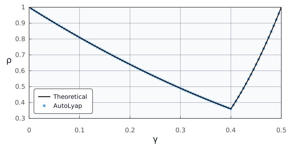
The computed value `rho (AutoLyap)` matches (up to solver numerical
tolerances) the theoretical rate expression for gradient methods; see
[[Pol63](https://autolyap.github.io/quick_start/#id164 "B. T. Polyak. Gradient methods for the minimisation of functionals. USSR Computational Mathematics and Mathematical Physics, 3(4):864–878, 1963. doi:10.1016/0041-5553(63)90382-3.")]:
\[\|x^k - x^\star\|^2 \in \mathcal{O}(\rho^k) \quad \textup{ as } \quad k\to\infty, \qquad
\rho = \max\{|1-\gamma L|,\;|1-\gamma\mu|\}^2,\]
where \(x^\star \in \Argmin_{x \in \calH} f(x)\).
Equivalently,
\[\|x^k - x^\star\| \in \mathcal{O}\!\left(\max\{|1-\gamma L|,\;|1-\gamma\mu|\}^k\right)
\quad \textup{ as } \quad k\to\infty.\]
Sweeping over 100 values of \(\gamma\) up to \(2/L\) gives the plot
below, with the endpoint included as the limiting \(\rho=1\) reference,
the theoretical rate in black, and AutoLyap certificates as blue dots.
[](https://autolyap.github.io/_images/gradient_method_rho_vs_gamma.svg)
## Iteration-dependent example: The optimized gradient method
### Problem setup
For background on the optimized gradient method, see
[[KF15](https://autolyap.github.io/quick_start/#id110 "Donghwan Kim and Jeffrey A. Fessler. Optimized first-order methods for smooth convex minimization. Mathematical Programming, 159(1-2):81–107, October 2015. doi:10.1007/s10107-015-0949-3.")].
Consider the unconstrained minimization problem
\[\minimize_{x \in \calH} f(x),\]
where \(f : \calH \to \reals\) is convex and \(L\)-smooth with
\(L>0\).
For initial points \(x^0, y^0 \in \calH\) and iteration budget
\(K \in \mathbb{N}\), the optimized gradient method updates as
\[\begin{split}(\forall k \in \llbracket 0, K-1 \rrbracket)\quad
\left[
\begin{aligned}
y^{k+1} &= x^k - \frac{1}{L}\nabla f(x^k), \\
x^{k+1} &= y^{k+1}
+ \frac{\theta_k - 1}{\theta_{k+1}}(y^{k+1} - y^k)
+ \frac{\theta_k}{\theta_{k+1}}(y^{k+1} - x^k).
\end{aligned}
\right.\end{split}\]
\[\begin{split}\theta_k =
\begin{cases}
1, & \text{if } k = 0, \\
\dfrac{1 + \sqrt{1 + 4\theta_{k-1}^2}}{2},
& \text{if } k \in \llbracket 1, K-1 \rrbracket, \\
\dfrac{1 + \sqrt{1 + 8\theta_{k-1}^2}}{2},
& \text{if } k = K.
\end{cases}\end{split}\]
In this example, we search for the smallest AutoLyap certificate constant
\(c_K\) such that
\[f(x^K)-f(x^\star)\le c_K\|x^0-x^\star\|^2,\]
where \(x^\star \in \Argmin_{x \in \calH} f(x)\).
### Model the problem in AutoLyap and search for the smallest c\_K
- \(f\) is modeled by
[`SmoothConvex`](https://autolyap.github.io/function_classes/#autolyap.problemclass.SmoothConvex "autolyap.problemclass.SmoothConvex").
- The optimization problem is represented by
[`InclusionProblem`](https://autolyap.github.io/problem_class/#autolyap.problemclass.InclusionProblem "autolyap.problemclass.InclusionProblem").
- The update rule is represented by
[`OptimizedGradientMethod`](https://autolyap.github.io/concrete_algorithms/#autolyap.algorithms.OptimizedGradientMethod "autolyap.algorithms.OptimizedGradientMethod").
- Initial-horizon parameters are obtained with
[`IterationDependent.get_parameters_distance_to_solution`](https://autolyap.github.io/iteration_dependent_analysis/#autolyap.IterationDependent.get_parameters_distance_to_solution "autolyap.IterationDependent.get_parameters_distance_to_solution").
- Final-horizon function-value parameters are obtained with
[`IterationDependent.get_parameters_function_value_suboptimality`](https://autolyap.github.io/iteration_dependent_analysis/#autolyap.IterationDependent.get_parameters_function_value_suboptimality "autolyap.IterationDependent.get_parameters_function_value_suboptimality").
- The certificate constant is computed with
[`IterationDependent.search_lyapunov`](https://autolyap.github.io/iteration_dependent_analysis/#autolyap.IterationDependent.search_lyapunov "autolyap.IterationDependent.search_lyapunov").
### Run the iteration-dependent analysis
```python
from autolyap.algorithms import OptimizedGradientMethod
from autolyap import SolverOptions
from autolyap.problemclass import InclusionProblem, SmoothConvex
from autolyap.iteration_dependent import IterationDependent
L = 1.0
K = 5
problem = InclusionProblem([SmoothConvex(L)])
algorithm = OptimizedGradientMethod(L=L, K=K)
solver_options = SolverOptions(backend="mosek_fusion") # requires `autolyap[mosek]`
# License-free option:
# solver_options = SolverOptions(backend="cvxpy", cvxpy_solver="CLARABEL")
Q_0, q_0 = IterationDependent.get_parameters_distance_to_solution(
algorithm,
0,
i=1,
j=1,
)
Q_K, q_K = IterationDependent.get_parameters_function_value_suboptimality(
algorithm,
K,
)
result = IterationDependent.search_lyapunov(
problem,
algorithm,
K,
Q_0,
Q_K,
q_0=q_0,
q_K=q_K,
solver_options=solver_options,
)
if result["status"] != "feasible":
raise RuntimeError("No feasible chained Lyapunov certificate for this setup.")
c_K = result["c_K"]
certificate = result["certificate"]
Q_sequence = certificate["Q_sequence"] # [Q_0, Q_1, ..., Q_K]
q_sequence = certificate["q_sequence"] # [q_0, q_1, ..., q_K] or None
theta_K = algorithm.compute_theta(K, K)
c_K_theory_value = L / (2.0 * theta_K ** 2)
print(f"c_K (AutoLyap): {c_K:.6e}")
print(f"c_K (theory): {c_K_theory_value:.6e}")
```
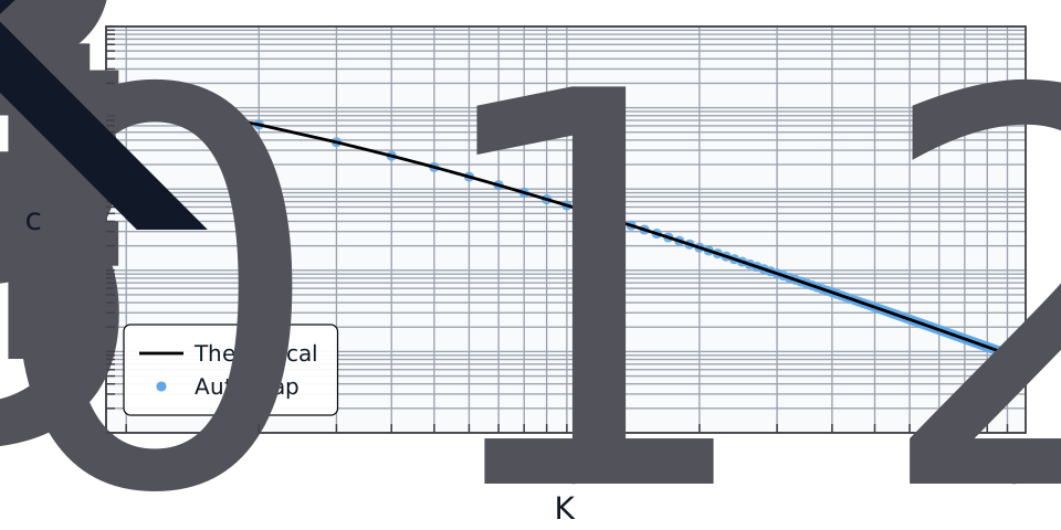
The computed value `c_K (AutoLyap)` matches (up to solver numerical
tolerances) the theoretical horizon-`K` expression:
\[f(x^K) - f(x^\star) \le c_K\,\|x^0 - x^\star\|^2, \qquad
c_K = \frac{L}{2\theta_K^2}.\]
where \(x^\star \in \Argmin_{x \in \calH} f(x)\).
In particular,
\[f(x^K) - f(x^\star) \in \mathcal{O}\!\left(\frac{1}{\theta_K^2}\right)
\quad \textup{ as } \quad K\to\infty,
\qquad
f(x^K) - f(x^\star) \in \mathcal{O}\!\left(\frac{1}{K^2}\right)
\quad \textup{ as } \quad K\to\infty.\]
Sweeping over \(K \in \llbracket 1, 100\rrbracket\) gives the plot below, with
the theoretical bound in black and AutoLyap certificates as blue dots.
[](https://autolyap.github.io/_images/optimized_gradient_method_c_vs_K_loglog.svg)
## What to inspect
- `status`: one of `feasible`, `infeasible`, or `not_solved`.
- `solve_status`: backend-specific raw solver status (or `solver_error` / `optimize_error`).
- `rho` (iteration-independent) or `c_K` (iteration-dependent): the main scalar output.
- `certificate`: Matrices and vectors that parameterize the Lyapunov certificate.
## Verbosity diagnostics
All three SDP entry points support a `verbosity` argument:
- [`IterationIndependent.search_lyapunov`](https://autolyap.github.io/iteration_independent_analysis/#autolyap.IterationIndependent.search_lyapunov "autolyap.IterationIndependent.search_lyapunov")
- [`IterationIndependent.LinearConvergence.bisection_search_rho`](https://autolyap.github.io/iteration_independent_analysis/#autolyap.IterationIndependent.LinearConvergence.bisection_search_rho "autolyap.IterationIndependent.LinearConvergence.bisection_search_rho")
- [`IterationDependent.search_lyapunov`](https://autolyap.github.io/iteration_dependent_analysis/#autolyap.IterationDependent.search_lyapunov "autolyap.IterationDependent.search_lyapunov")
Set:
- `verbosity=1` for concise diagnostic summaries (default).
- `verbosity=0` for silent mode.
- `verbosity=2` for detailed per-constraint/per-iteration diagnostics.
The diagnostic summary reports:
- nonnegativity checks on constrained scalars,
- PSD checks via minimum eigenvalues of constrained matrices,
- equality-constraint residuals (`max_abs_residual` and `l2_residual`).
Example:
```python
result = IterationIndependent.search_lyapunov(
problem,
algorithm,
P,
T,
p=p,
t=t,
rho=1.0,
solver_options=solver_options,
verbosity=1, # or 2 for detailed diagnostics
)
```
## Next
- For theoretical foundations, see [Theory](https://autolyap.github.io/theory/).
- For more worked walkthroughs, see [Examples](https://autolyap.github.io/examples/).
- For the full API, see [API reference](https://autolyap.github.io/api_reference/).
## References
[[KF15](https://autolyap.github.io/quick_start/#id3)]
Donghwan Kim and Jeffrey A. Fessler. Optimized first-order methods for smooth convex minimization. *Mathematical Programming*, 159(1-2):81–107, October 2015. [doi:10.1007/s10107-015-0949-3](https://doi.org/10.1007/s10107-015-0949-3).
[[Pol63](https://autolyap.github.io/quick_start/#id1)]
B. T. Polyak. Gradient methods for the minimisation of functionals. *USSR Computational Mathematics and Mathematical Physics*, 3(4):864–878, 1963. [doi:10.1016/0041-5553(63)90382-3](https://doi.org/10.1016/0041-5553(63)90382-3).
TeX macro definitions used in this page:
```latex
\newcommand{\Argmin}{\operatorname*{Argmin}}
\newcommand{\calH}{\mathcal{H}}
\newcommand{\llbracket}{\lbrack\!\lbrack}
\newcommand{\minimize}{\operatorname*{minimize}}
\newcommand{\naturals}{\mathbb{N}_{0}}
\newcommand{\reals}{\mathbb{R}}
\newcommand{\rrbracket}{\rbrack\!\rbrack}
```