Canonical HTML: https://autolyap.github.io/examples/proximal_point/
Documentation version: 0.2.1

<a id="the-proximal-point-method"></a>



# The proximal point method

<a id="problem-setup"></a>



## Problem setup

Consider the unconstrained minimization problem


\[\minimize_{x \in \calH} f(x) \quad \iff \quad \text{find } x \in \calH \text{ such that } 0 \in \partial f(x),\]

where \(f : \calH \to \reals\) is \(\mu\)-strongly convex with
\(\mu>0\).

For an initial point \(x^0 \in \calH\) and step size
\(\gamma \in \reals_{++}\), the proximal point update
<a id="id1"></a>[[Mar70](https://autolyap.github.io/examples/proximal_point/#id170 "B. Martinet. Brève communication. Régularisation d'inéquations variationnelles par approximations successives. Revue française d'informatique et de recherche opérationnelle. Série rouge, 4(R3):154–158, 1970. doi:10.1051/m2an/197004R301541."), [Mor65](https://autolyap.github.io/examples/proximal_point/#id171 "Jean-Jacques Moreau. Proximité et dualité dans un espace hilbertien. Bulletin de la Société Mathématique de France, 93:273–299, 1965. doi:10.24033/bsmf.1625."), [Roc76](https://autolyap.github.io/examples/proximal_point/#id169 "R. Tyrrell Rockafellar. Monotone operators and the proximal point algorithm. SIAM Journal on Control and Optimization, 14(5):877–898, 1976. doi:10.1137/0314056.")] is


\[(\forall k \in \naturals)\quad
x^{k+1} = \prox_{\gamma f}(x^k).\]

In this example, we search for the smallest contraction factor
\(\rho\in[0,1)\) provable using AutoLyap such that


\[\|x^{k+1} - x^\star\|^2 \in \mathcal{O}(\rho^k) \quad \textup{ as } \quad k\to\infty,\]

where


\[x^\star \in \Argmin_{x \in \calH} f(x).\]

<a id="model-the-problem-in-autolyap-and-search-for-the-smallest-rho"></a>



## Model the problem in AutoLyap and search for the smallest rho

- \(f\) is modeled by
  [`StronglyConvex`](https://autolyap.github.io/function_classes/#autolyap.problemclass.StronglyConvex "autolyap.problemclass.StronglyConvex").
- The optimization problem is represented by
  [`InclusionProblem`](https://autolyap.github.io/problem_class/#autolyap.problemclass.InclusionProblem "autolyap.problemclass.InclusionProblem").
- The update rule is represented by
  [`ProximalPoint`](https://autolyap.github.io/concrete_algorithms/#autolyap.algorithms.ProximalPoint "autolyap.algorithms.ProximalPoint").
- Distance-to-solution parameters are obtained with
  [`IterationIndependent.LinearConvergence.get_parameters_distance_to_solution`](https://autolyap.github.io/iteration_independent_analysis/#autolyap.IterationIndependent.LinearConvergence.get_parameters_distance_to_solution "autolyap.IterationIndependent.LinearConvergence.get_parameters_distance_to_solution").
- The contraction factor is searched with
  [`IterationIndependent.LinearConvergence.bisection_search_rho`](https://autolyap.github.io/iteration_independent_analysis/#autolyap.IterationIndependent.LinearConvergence.bisection_search_rho "autolyap.IterationIndependent.LinearConvergence.bisection_search_rho").

<a id="run-the-iteration-independent-analysis"></a>



## Run the iteration-independent analysis

This example uses the MOSEK Fusion backend (`backend="mosek_fusion"`).
Install the optional MOSEK dependency first:



```bash
pip install "autolyap[mosek]"
```





```python
from autolyap import SolverOptions
from autolyap.algorithms import ProximalPoint
from autolyap.problemclass import InclusionProblem, StronglyConvex
from autolyap.iteration_independent import IterationIndependent

mu = 1.0
gamma = 0.6

problem = InclusionProblem([StronglyConvex(mu)])
algorithm = ProximalPoint(gamma=gamma)
solver_options = SolverOptions(backend="mosek_fusion")
# License-free option:
# solver_options = SolverOptions(backend="cvxpy", cvxpy_solver="CLARABEL")

# Build V(P, p, k) and R(T, t, k) for distance-to-solution analysis.
P, p, T, t = IterationIndependent.LinearConvergence.get_parameters_distance_to_solution(
    algorithm
)

result = IterationIndependent.LinearConvergence.bisection_search_rho(
    problem,
    algorithm,
    P,
    T,
    p=p,
    t=t,
    S_equals_T=True,
    s_equals_t=True,
    remove_C3=True,
    solver_options=solver_options,
)

if result["status"] != "feasible":
    raise RuntimeError("No feasible Lyapunov certificate in the requested rho interval.")

rho_autolyap = result["rho"]
rho_theory = (1.0 / (1.0 + gamma * mu)) ** 2

print(f"rho (AutoLyap): {rho_autolyap:.8f}")
print(f"rho (theory):   {rho_theory:.8f}")
```



What to inspect in `result`:

- `result["status"]`: `feasible`, `infeasible`, or `not_solved`.
- `result["solve_status"]`: raw backend status.
- `result["rho"]`: certified contraction factor when feasible.
- `result["certificate"]`: Lyapunov certificate matrices/scalars.

The computed value `rho (AutoLyap)` matches (up to solver numerical
tolerances) the theoretical rate expression in <a id="id2"></a>[[Roc76](https://autolyap.github.io/examples/proximal_point/#id169 "R. Tyrrell Rockafellar. Monotone operators and the proximal point algorithm. SIAM Journal on Control and Optimization, 14(5):877–898, 1976. doi:10.1137/0314056.")],
i.e.,


\[\|x^{k+1} - x^\star\|^2 \in \mathcal{O}(\rho^k) \quad \textup{ as } \quad k\to\infty,\]

where


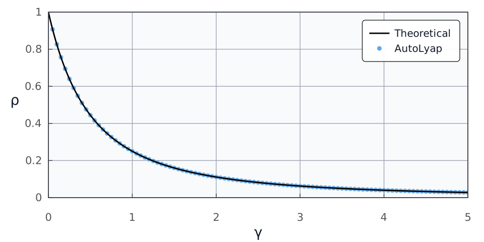
\[\rho = \left(\frac{1}{1+\gamma\mu}\right)^2,\]

and


\[x^\star \in \Argmin_{x \in \calH} f(x).\]

Equivalently,


\[\|x^{k+1} - x^\star\| \in \mathcal{O}\!\left(\left(\frac{1}{1+\gamma\mu}\right)^k\right)
\quad \textup{ as } \quad k\to\infty.\]

Sweeping over 100 values of \(\gamma\) on \(0 < \gamma \le 5\) gives
the plot below, with the theoretical rate in black and AutoLyap certificates
as blue dots.

[![Proximal-point rho versus gamma with theoretical line and AutoLyap points.](https://autolyap.github.io/_images/proximal_point_rho_vs_gamma.svg)](https://autolyap.github.io/_images/proximal_point_rho_vs_gamma.svg)

<a id="references"></a>



## References

<a id="id3"></a>



<a id="id170"></a>



[[Mar70](https://autolyap.github.io/examples/proximal_point/#id1)]

B. Martinet. Brève communication. Régularisation d'inéquations variationnelles par approximations successives. *Revue française d'informatique et de recherche opérationnelle. Série rouge*, 4(R3):154–158, 1970. [doi:10.1051/m2an/197004R301541](https://doi.org/10.1051/m2an/197004R301541).

<a id="id171"></a>



[[Mor65](https://autolyap.github.io/examples/proximal_point/#id1)]

Jean-Jacques Moreau. Proximité et dualité dans un espace hilbertien. *Bulletin de la Société Mathématique de France*, 93:273–299, 1965. [doi:10.24033/bsmf.1625](https://doi.org/10.24033/bsmf.1625).

<a id="id169"></a>



[Roc76]
([1](https://autolyap.github.io/examples/proximal_point/#id1),[2](https://autolyap.github.io/examples/proximal_point/#id2))

R. Tyrrell Rockafellar. Monotone operators and the proximal point algorithm. *SIAM Journal on Control and Optimization*, 14(5):877–898, 1976. [doi:10.1137/0314056](https://doi.org/10.1137/0314056).

TeX macro definitions used in this page:

```latex
\newcommand{\Argmin}{\operatorname*{Argmin}}
\newcommand{\calH}{\mathcal{H}}
\newcommand{\minimize}{\operatorname*{minimize}}
\newcommand{\naturals}{\mathbb{N}_{0}}
\newcommand{\prox}{{\rm{prox}}}
\newcommand{\reals}{\mathbb{R}}
```