Canonical HTML: https://autolyap.github.io/examples/nesterov_fast_gradient/
Documentation version: 0.2.1

<a id="nesterov-s-fast-gradient-method"></a>



# Nesterov’s fast gradient method

<a id="problem-setup"></a>



## Problem setup

Consider minimizing a convex and \(L\)-smooth function
\(f : \calH \to \reals\), with \(L > 0\).

For initial points \(x^{-1},x^0 \in \calH\), step size
\(\gamma \in \reals_{++}\), and \(\lambda_0 = 1\), Nesterov’s fast
gradient method is


\[\begin{split}(\forall k \in \naturals)\quad
\left[
\begin{aligned}
y^k &= x^k + \delta_k(x^k - x^{k-1}), \\
x^{k+1} &= y^k - \gamma \nabla f(y^k),\\
\delta_k &= \frac{\lambda_k - 1}{\lambda_{k+1}},\\
\lambda_{k+1} &= \frac{1 + \sqrt{1 + 4\lambda_k^2}}{2}.
\end{aligned}
\right.\end{split}\]

For \(\gamma = 1/L\), the classical bound in <a id="id1"></a>[[Nes83](https://autolyap.github.io/examples/nesterov_fast_gradient/#id145 "Yurii Nesterov. A method for solving the convex programming problem with convergence rate o(1/k^2). Doklady Akademii Nauk SSSR, 269(3):543–547, 1983.")] is


\[f(x^K)-f(x^\star)\le\frac{L}{2\lambda_K^2}\|x^0-x^\star\|^2
\le\frac{2L}{(K+2)^2}\|x^0-x^\star\|^2,\]

where \(x^\star \in \Argmin_{x \in \calH} f(x)\).

In this example, we compute the smallest AutoLyap certificate constant
\(c_K\) such that


\[f(x^K)-f(x^\star)\le c_K\|x^0-x^\star\|^2.\]

<a id="run-the-iteration-dependent-analysis"></a>



## Run the iteration-dependent analysis

This example uses the MOSEK Fusion backend (`backend="mosek_fusion"`).
Install the optional MOSEK dependency first:



```bash
pip install "autolyap[mosek]"
```





```python
from autolyap import IterationDependent, SolverOptions
from autolyap.algorithms import NesterovFastGradientMethod
from autolyap.problemclass import InclusionProblem, SmoothConvex

L = 1.0
K = 10

problem = InclusionProblem([SmoothConvex(L)])
solver_options = SolverOptions(backend="mosek_fusion")

# Nesterov fast gradient method
nfgm = NesterovFastGradientMethod(gamma=1.0 / L)

# Use j=2 to select x^k; j=1 corresponds to y^k.
Q_0_nf, q_0_nf = IterationDependent.get_parameters_distance_to_solution(
    nfgm, 0, i=1, j=2
)
Q_K_nf, q_K_nf = IterationDependent.get_parameters_function_value_suboptimality(
    nfgm, K, j=2
)

result_nf = IterationDependent.search_lyapunov(
    problem,
    nfgm,
    K,
    Q_0_nf,
    Q_K_nf,
    q_0=q_0_nf,
    q_K=q_K_nf,
    solver_options=solver_options,
)
if result_nf["status"] != "feasible":
    raise RuntimeError("No feasible chained Lyapunov certificate for Nesterov FGM.")

def lambda_k(k: int) -> float:
    lam = 1.0
    for _ in range(k):
        lam = 0.5 * (1.0 + (1.0 + 4.0 * lam * lam) ** 0.5)
    return lam

lam_K = lambda_k(K)
c_K_nf = result_nf["c_K"]
c_K_nesterov = L / (2.0 * lam_K**2)
c_K_nesterov_simple = 2.0 * L / ((K + 2.0) ** 2)

print(f"Nesterov FGM c_K (AutoLyap):            {c_K_nf:.6e}")
print(f"Nesterov FGM c_K (L/(2*lambda_K^2)):    {c_K_nesterov:.6e}")
print(f"Nesterov FGM c_K (2L/(K+2)^2):          {c_K_nesterov_simple:.6e}")
```



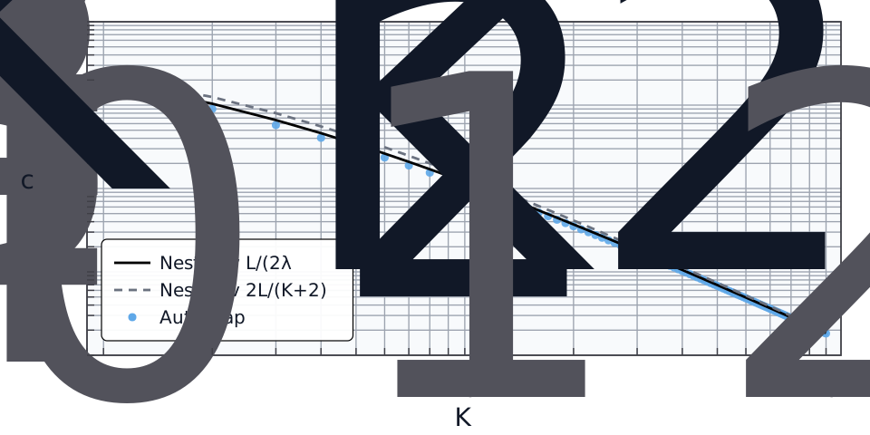
Sweeping over \(K \in \llbracket 1, 100\rrbracket\) gives the log-log plot
below, with the two classical bounds as lines and AutoLyap certificates as blue
dots.

[![Nesterov-fast c_K versus K in log-log scale with classical bounds and AutoLyap points.](https://autolyap.github.io/_images/nesterov_fast_gradient_method_c_vs_K_loglog.svg)](https://autolyap.github.io/_images/nesterov_fast_gradient_method_c_vs_K_loglog.svg)

<a id="references"></a>



## References

<a id="id2"></a>



<a id="id145"></a>



[[Nes83](https://autolyap.github.io/examples/nesterov_fast_gradient/#id1)]

Yurii Nesterov. A method for solving the convex programming problem with convergence rate o(1/k^2). *Doklady Akademii Nauk SSSR*, 269(3):543–547, 1983.

TeX macro definitions used in this page:

```latex
\newcommand{\Argmin}{\operatorname*{Argmin}}
\newcommand{\calH}{\mathcal{H}}
\newcommand{\llbracket}{\lbrack\!\lbrack}
\newcommand{\naturals}{\mathbb{N}_{0}}
\newcommand{\reals}{\mathbb{R}}
\newcommand{\rrbracket}{\rbrack\!\rbrack}
```