Canonical HTML: https://autolyap.github.io/examples/define_your_own_algorithm/proximal_gradient_method/
Documentation version: 0.2.1

<a id="the-proximal-gradient-method"></a>



# The proximal gradient method

This example shows how to define a custom
[`Algorithm`](https://autolyap.github.io/base_algorithms/#autolyap.algorithms.Algorithm "autolyap.algorithms.Algorithm") for proximal gradient and
then analyze its convergence with AutoLyap.

We consider the composite minimization problem


\[\minimize_{x \in \calH} \; f(x) + g(x) \quad  \iff \quad \text{find } x \in \calH \text{ such that } 0 \in \nabla f(x) + \partial g(x),\]

where \(f\) is \(L\)-smooth and \(\mu\)-strongly convex with
\(0<\mu<L\), and \(g\) is proper, lower semicontinuous, and convex.

For an initial point \(x^0 \in \calH\) and step size
\(\gamma \in \reals_{++}\) with \(0 < \gamma < 2/L\), the proximal
gradient method is given by

<a id="equation-eq-proximal-gradient-update"></a>




(1)\[(\forall k \in \naturals)\quad
x^{k+1} = \prox_{\gamma g}\!\left(x^k - \gamma \nabla f(x^k)\right).\]

The analysis goal is to search for the smallest contraction factor provable via
AutoLyap:


\[\|x^k - x^\star\|^2 \in \mathcal{O}(\rho^k) \quad \textup{ as } \quad k\to\infty,\]

where


\[x^\star \in \Argmin_{x \in \calH} \bigl(f(x)+g(x)\bigr).\]

<a id="step-1-problem-class"></a>



## Step 1: Problem class

Let \((\calH,\langle\cdot,\cdot\rangle)\) be a real Hilbert space with canonical norm
\(\|\cdot\|\).

Use the inclusion form


\[\text{find } y \in \calH \text{ such that } 0 \in \sum_{i \in \IndexFunc} \partial f_i(y)
+ \sum_{i \in \IndexOp} G_i(y),\]

with two functional components and no operator component:

- \(f_1 = f\), where


\[f:\calH \to \mathbb{R}\]

  is \(L\)-smooth and \(\mu\)-strongly convex
  (\(0 < \mu < L < +\infty\)).
- \(f_2 = g\), where


\[g:\calH \to \mathbb{R}\cup\{+\infty\}\]

  is proper, lower semicontinuous, and convex, with subdifferential


\[\partial g:\calH \rightrightarrows \calH.\]
- \(\IndexFunc = \{1,2\}\) and \(\IndexOp = \emptyset\).

Equivalently,


\[\text{find } y \in \calH \text{ such that } 0 \in \nabla f(y) + \partial g(y).\]

<a id="step-2-update-rule-and-equivalent-inclusion"></a>



## Step 2: Update rule and equivalent inclusion

The proximal-gradient update is given in [(1)](https://autolyap.github.io/examples/define_your_own_algorithm/proximal_gradient_method/#equation-eq-proximal-gradient-update). Applying the proximal-operator optimality condition gives the equivalent inclusion


\[\frac{x^k - x^{k+1}}{\gamma} - \nabla f(x^k) \in \partial g(x^{k+1})\]

which can be rearranged as


\[x^{k+1} \in x^k - \gamma \nabla f(x^k) - \gamma \partial g(x^{k+1}).\]

<a id="step-3-state-space-representation"></a>



## Step 3: State-space representation

Match the base representation used by
[`Algorithm`](https://autolyap.github.io/base_algorithms/#autolyap.algorithms.Algorithm "autolyap.algorithms.Algorithm")


\[\begin{split}\begin{aligned}
\bx^{k+1} &= (A_k \kron \Id)\bx^k + (B_k \kron \Id)\bu^k,\\
\by^k &= (C_k \kron \Id)\bx^k + (D_k \kron \Id)\bu^k,\\
(\bu_i^k)_{i \in \IndexFunc} &\in \prod_{i \in \IndexFunc} \boldsymbol{\partial}\bfcn_i(\by_i^k)
\end{aligned}\end{split}\]

with


\[\begin{split}\begin{aligned}
\bx^k &= x^k,\\
\bu^k &= \left(\nabla f(x^k),\, \frac{x^k - x^{k+1}}{\gamma} - \nabla f(x^k)\right),\\
\by^k &= (x^k, x^{k+1}),\\
\boldsymbol{\partial}\bfcn_1 &: \calH \rightrightarrows \calH : y \mapsto  \partial f(y) = \{\nabla f(y)\},\\
\boldsymbol{\partial}\bfcn_2 &: \calH \rightrightarrows \calH : y \mapsto  \partial g(y).
\end{aligned}\end{split}\]

and the matrices


\[\begin{split}\begin{aligned}
A_k &= \begin{bmatrix} 1 \end{bmatrix}, &
B_k &= \begin{bmatrix} -\gamma & -\gamma \end{bmatrix}, \\
C_k &=
\begin{bmatrix}
1 \\
1
\end{bmatrix}, &
D_k &=
\begin{bmatrix}
0 & 0 \\
-\gamma & -\gamma
\end{bmatrix}.
\end{aligned}\end{split}\]

<a id="step-4-implement-the-custom-algorithm"></a>



## Step 4: Implement the custom algorithm



```python
import numpy as np
from typing import Tuple

from autolyap.algorithms import Algorithm

class ProximalGradientMethod(Algorithm):
    def __init__(self, gamma):
        super().__init__(n=1, m=2, m_bar_is=[1, 1], I_func=[1, 2], I_op=[])
        self.set_gamma(gamma)

    def set_gamma(self, gamma: float) -> None:
        self.gamma = gamma

    def get_ABCD(self, k: int) -> Tuple[np.ndarray, np.ndarray, np.ndarray, np.ndarray]:
        A = np.array([[1.0]])
        B = np.array([[-self.gamma, -self.gamma]])
        C = np.array([[1.0], [1.0]])
        D = np.array([
            [0.0, 0.0],
            [-self.gamma, -self.gamma],
        ])
        return A, B, C, D
```



<a id="step-5-build-inclusionproblem-and-run-the-analysis"></a>



## Step 5: Build [`InclusionProblem`](https://autolyap.github.io/problem_class/#autolyap.problemclass.InclusionProblem "autolyap.problemclass.InclusionProblem") and run the analysis

This example uses the MOSEK Fusion backend (`backend="mosek_fusion"`).
Install the optional MOSEK dependency first:



```bash
pip install "autolyap[mosek]"
```





```python
from autolyap import IterationIndependent, SolverOptions
from autolyap.problemclass import Convex, InclusionProblem, SmoothStronglyConvex


def validate_parameters(mu: float, L: float, gamma: float) -> None:
    if not (0.0 < mu < L):
        raise ValueError(
            f"Invalid parameters: require 0 < mu < L. Got mu={mu}, L={L}."
        )

    gamma_max = 2.0 / L
    if not (0.0 < gamma < gamma_max):
        raise ValueError(
            f"Invalid parameters: require 0 < gamma < 2/L. Got gamma={gamma}, 2/L={gamma_max}."
        )


mu = 1.0
L = 4.0
gamma = 2.0 / (L + mu)
validate_parameters(mu=mu, L=L, gamma=gamma)

problem = InclusionProblem([
    SmoothStronglyConvex(mu, L),    # component i=1: f
    Convex(),                       # component i=2: g
])
algorithm = ProximalGradientMethod(gamma=gamma)
solver_options = SolverOptions(backend="mosek_fusion")

P, p, T, t = IterationIndependent.LinearConvergence.get_parameters_distance_to_solution(
    algorithm,
    i=1,
    j=1,
)

result = IterationIndependent.LinearConvergence.bisection_search_rho(
    problem,
    algorithm,
    P,
    T,
    p=p,
    t=t,
    S_equals_T=True,
    s_equals_t=True,
    remove_C3=True,
    solver_options=solver_options,
)

if result["status"] != "feasible":
    raise RuntimeError("No feasible Lyapunov certificate in the requested rho interval.")

rho_autolyap = result["rho"]
rho_taylor = max(abs(1.0 - L * gamma), abs(1.0 - mu * gamma)) ** 2

print(f"rho (AutoLyap):  {rho_autolyap:.8f}")
print(f"rho (theory):    {rho_taylor:.8f}")
```



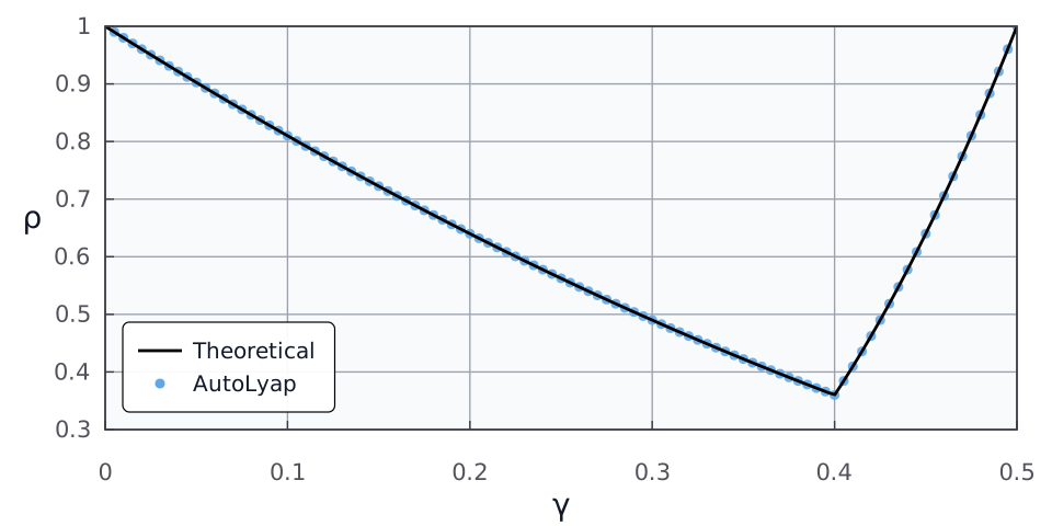
The computed value `rho (AutoLyap)` matches (up to solver numerical
tolerances) the closed-form theoretical rate expression in <a id="id1"></a>[[THG18](https://autolyap.github.io/examples/define_your_own_algorithm/proximal_gradient_method/#id193 "Adrien B. Taylor, Julien M. Hendrickx, and Francois Glineur. The exact worst-case convergence rate of the proximal gradient method for composite convex optimization. Journal of Optimization Theory and Applications, 178(2):455–476, 2018. doi:10.1007/s10957-018-1298-1.")],
Theorem 2.1, i.e.,


\[\|x^k - x^\star\|^2 \in \mathcal{O}(\rho^k) \quad \textup{ as } \quad k\to\infty, \qquad
\rho = \max\{|1-\gamma L|,\;|1-\gamma\mu|\}^2,\]

where \(x^\star \in \Argmin_{x \in \calH} \bigl(f(x)+g(x)\bigr)\).

Equivalently,


\[\|x^k - x^\star\| \in \mathcal{O}\!\left(\max\{|1-\gamma L|,\;|1-\gamma\mu|\}^k\right)
\quad \textup{ as } \quad k\to\infty.\]

Sweeping over 100 values of \(\gamma\) on \(0 < \gamma < 2/L\) gives
the plot below, with the theoretical rate in black and AutoLyap certificates
as blue dots.

[![Proximal-gradient rho versus gamma with theoretical line and AutoLyap points.](https://autolyap.github.io/_images/proximal_gradient_rho_vs_gamma.svg)](https://autolyap.github.io/_images/proximal_gradient_rho_vs_gamma.svg)

<a id="references"></a>



## References

<a id="id2"></a>



<a id="id193"></a>



[[THG18](https://autolyap.github.io/examples/define_your_own_algorithm/proximal_gradient_method/#id1)]

Adrien B. Taylor, Julien M. Hendrickx, and Francois Glineur. The exact worst-case convergence rate of the proximal gradient method for composite convex optimization. *Journal of Optimization Theory and Applications*, 178(2):455–476, 2018. [doi:10.1007/s10957-018-1298-1](https://doi.org/10.1007/s10957-018-1298-1).

TeX macro definitions used in this page:

```latex
\newcommand{\Argmin}{\operatorname*{Argmin}}
\newcommand{\Id}{\operatorname*{Id}}
\newcommand{\IndexFunc}{\mathcal{I}_{\textup{func}}}
\newcommand{\IndexOp}{\mathcal{I}_{\textup{op}}}
\newcommand{\bfcn}{\mathbf{f}}
\newcommand{\bu}{\mathbf{u}}
\newcommand{\bx}{\mathbf{x}}
\newcommand{\by}{\mathbf{y}}
\newcommand{\calH}{\mathcal{H}}
\newcommand{\kron}{\otimes}
\newcommand{\minimize}{\operatorname*{minimize}}
\newcommand{\naturals}{\mathbb{N}_{0}}
\newcommand{\prox}{{\rm{prox}}}
\newcommand{\reals}{\mathbb{R}}
```